In this post, we explain how Solr calculates the relatedness score.
Relatedness is an excellent tool to look at the semantic knowledge graphs in your index corpus. How to retrieve the relatedness score in Solr is described in more details here in the Solr manual. There you will also find the link to the paper with theory about “The Semantic Knowledge Graph” that we’ll also use and refer to in this post.
We wanted to understand the mathematics behind the relatedness function in Solr: What is the score? How does it relate to the z-score? And what sigmoid function is used to bring back the score between -1 and 1. Googling didn’t brought back the details we were after, so we deep-dived ourselves.
For this case study’s example, we are using the chorus project ‘Towards an open source tool stack for e-commerce search‘ with its e-commerce data. All details can be found on its github pages here.
We will be investigating the returned relatedness scores of the product types that are brought back for the query “coffee”. These scores are:
Product type with relatedness score |
|---|
Drip coffee maker : 0.84873 |
This table shows the summary of the Solr request for our relatedness score calculation case. We’ll get this data via the following Solr request (here as curl request that you can copy/past if you like to do the hands-on):
curl -X POST --location "http://localhost:8983/solr/ecommerce/select" -H "Content-Type: application/json" -d '{
  "params": {
    "fore": "{!type=$defType qf=$qf v=$q}",
    "back": "{!type=$defType qf=$qf v=*}",
    "rows": 0,
    "q": "coffee",
    "useParams": "default_algo"
  },
  "facet": {
    "related_values": {
      "type": "terms",
      "field": "filter_product_type",
      "sort": { "relatedness": "desc"},
      "facet": {
        "relatedness": {
          "type": "func",
          "func": "relatedness($fore,$back)"
        }
      }
    }
  }
}'
This brings back the following (clipped) response:
  "response": {
    "numFound": 203,
    ...
  },
  "facets": {
    "count": 203,
    "related_values": {
      "buckets": [
        {
          "val": "Drip coffee maker",
          "count": 68,
          "relatedness": {
            "relatedness": 0.84873,
            "foreground_popularity": 4.5E-4,
            "background_popularity": 4.5E-4
          }
        },
        {
          "val": "Pod coffee machine",
          "count": 63,
          "relatedness": {
            "relatedness": 0.84322,
            "foreground_popularity": 4.2E-4,
            "background_popularity": 4.2E-4
          }
        },
        {
          "val": "Espresso machine",
          "count": 19,
          "relatedness": {
            "relatedness": 0.64246,
            "foreground_popularity": 1.3E-4,
            "background_popularity": 2.1E-4
          }
        }, ...
In this response, we get additional information: foreground_popularity and backgroud_popularity. The foreground_popularity refers to the popularity of the bucket value in our foreground query (q=coffee). The background_popularity is the popularity of the bucket value in our background query (q=*).
The foreground and background popularities are the same for the first 2 bucket values in our example (“Drip coffee maker” and “Pod coffee machine”). The reason is simply because the “count” value is the same in the background (with q=*) as in the foreground (with q=coffee). We’ll elaborate on the 3rd bucket as that one has different values what makes the break down a bit more clear.
So for the “Espresso machine” bucket, we have a foreground count of 19. In order to be able to re-calculate all the figures, we still are missing 2 values that are available to Solr but not in our original response: the total count of our corpus (background query) and the count of our bucket in the background query.
In order to retrieve these values, we can just relaunch our solr request from above with the background query (q=*) instead of the foreground query (q=coffee) and looking at the facet for the field “filter_product_type” with value “Espresso machine”. This can be achieved with the below request:
curl -X POST --location "http://localhost:8983/solr/ecommerce/select" -H "Content-Type: application/json" -d '{
  "params": {
    "rows": 0,
    "q": "*",
    "useParams": "default_algo",
    "facet": true,
    "facet.field": "filter_product_type",
    "facet.matches": "Esp.*"
  }
}'
This gives the following response:
  "response": { "numFound": 150247, ... },
  "facet_counts": { ...  "facet_fields": { "filter_product_type": [ "Espresso machine", 31 ] ...
Now we have all info required for our popularity calculations.
Foreground popularity: 19 / 150247 = 0.00013 = 1.3E-04
Background popularity: 31 / 150247 = 0.00021 = 2.1E-04
Now we should have a look at the relatedness score.
Let’s start with the z-score as described in the paper:

Filling the parameters in the formula gives us our z-score:
| y | the number of documents containing both xi and xj | 19 |
| n | number of documents in our foreground document set | 203 |
| p | the probability of finding the term xj with tag tk in the background document set | 2.1E-04 |
| n*p | 0.04188 | |
| y-n*p | 18.95812 | |
| SQRT(n*p*(1-p)) | 0.2046355831 | |
| z | 92.64330 |
So far so good. We now have our z-score. The paper further describes:
“We normalize the z score using a sigmoid function to bring the scores in the range [−1, 1]. We call the normalized score the relatedness score between nodes where 1 means completely positively related (likely to always appear together), while 0 means no relatedness (just as likely as anything else to appear together), and -1 means completely negatively related (unlikely to appear together).”
2016 Trey Grainger, Khalifeh AlJadda, Mohammed Korayem, and Andries Smith: “The Semantic Knowledge Graph: A compact, auto-generated model for real-time traversal and ranking of any relationship within a domain”
So the question is what sigmoid function is applied to normalize the z-score?
The first candidate is the commonly used “logistic function” (more info on wiki):

Using this function would immediately return a value of 1 as all scores above 6 will return (a value close to) 1.
As our example shows, our z-score might vary in a range that is much wider than -6 to 6…
Hence a modification to our sigmoid function is needed to make it useful for a wider range of values. In order to be able to recalculate the values, we digged into the source code of the function in the solr repo.
Applying this logic to our example, we calculated the actual relatedness value for “Espresso machine“: 0.64246
| offset | scale | z’ = z+offset | z” = z’/(scale-ABS(z’)) | factor | z” * factor |
| -80 | 50 | 12.64 | 0.20 | 0.2 | 0.0404 |
| -30 | 30 | 62.64 | 0.68 | 0.2 | 0.1352 |
| 0 | 30 | 92.64 | 0.76 | 0.2 | 0.1511 |
| 30 | 30 | 122.64 | 0.80 | 0.2 | 0.1607 |
| 80 | 50 | 172.64 | 0.78 | 0.2 | 0.1551 |
| sum: | 0.64246 |
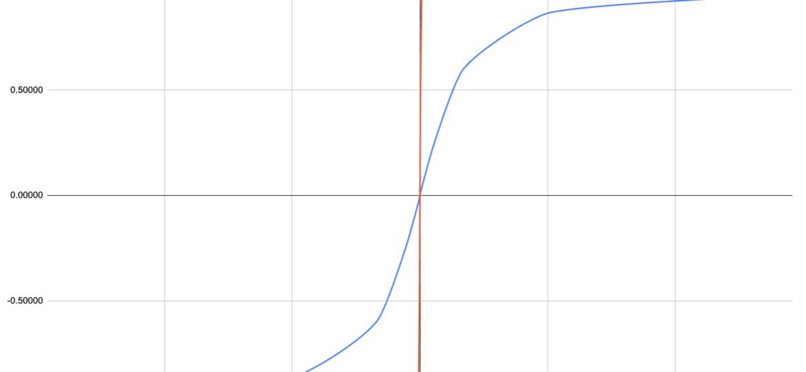
In order to make the sigmoid a bit more “understandable” and visible, we can look at the graph below that illustrates the difference between the solr sigmoid function and the logistic function.
This illustrates clearly how the solr sigmoid is able to derive a relatedness score between -1 and 1 while the incoming z-score can still hava a wide range of values.

We hope this helps other people that might want to understand the relatedness score in detail.
For more info, don’t hesitate to contact us.